Control System Design with Python

Introduction to Control Systems Engineering

Control systems engineering is a crucial field that deals with the analysis and design of systems that maintain desired behaviors through feedback mechanisms. Python provides powerful tools for control system analysis and design.

Key Python Libraries

The following libraries are essential for control systems engineering:

numpy - Numerical computations
- Efficient array operations
- Linear algebra functions
- Mathematical functions
control - Control systems analysis
- Transfer function creation and manipulation
- System analysis tools
- Control design methods
matplotlib - Data visualization
- 2D and 3D plotting
- Multiple plot types
- Customizable visualizations
sympy - Symbolic mathematics
- Symbolic calculations
- Equation solving
- Laplace transforms
scipy - Scientific computing
- Differential equation solvers
- Optimization tools
- Signal processing functions

Python Fundamentals for Control Systems

Basic Python Concepts

Python Syntax Overview

Python's clean and readable syntax makes it ideal for engineering applications:

# Basic variable assignments
x = 123.3
text = "Some text"
flag = True
print(f"x = {x}, text = {text}, flag = {flag}")

# Lists (similar to arrays in other languages)
x = [1, 2, 3, 4]
print("List x:", x)

Output:

x = 123.3, text = Some text, flag = True
List x: [1, 2, 3, 4]

NumPy for Numerical Computations

NumPy Arrays and Operations

NumPy provides efficient array operations essential for control systems:

import numpy as np

# Creating arrays
x = np.array([1, 2, 3, 4])
print("NumPy array x:", x)

# Arrays of zeros and ones
x = np.zeros(4)
y = np.ones((2, 2))
print("Array of zeros:", x)
print("2x2 array of ones:\n", y)

# Array operations
a = np.array([1, 2, 3])
b = np.array([4, 5, 6])
print("\nArray operations:")
print("a + b =", a + b)
print("a * b =", a * b)
print("a dot b =", np.dot(a, b))

Output:

NumPy array x: [1 2 3 4]
Array of zeros: [0. 0. 0. 0.]
2x2 array of ones:
 [[1. 1.]
  [1. 1.]]

Array operations:
a + b = [5 7 9]
a * b = [ 4 10 18]
a dot b = 32

Symbolic Mathematics with SymPy

Let's start with basic symbolic operations using a quadratic expression:

Consider the quadratic expression:

\[ f(x) = x^2 + 2x + 1 \]

In standard form:

\[ ax^2 + bx + c \text{ where } a=1, b=2, c=1 \]

Complete square form:

\[ (x + 1)^2 \]

Root:

\[ x = -1 \text{ (single root)} \]

Basic Symbolic Operations

import sympy as sp

# Define symbolic variable
x = sp.Symbol('x')

# Create and manipulate expressions
expr = x**2 + 2*x + 1
print("Original expression:", expr)

# Solve equation
eq = sp.Eq(expr, 0)
solution = sp.solve(eq, x)
print("\nSolving x^2 + 2x + 1 = 0:")
print("x =", solution)

Output:

Original expression: x**2 + 2*x + 1

Solving x^2 + 2x + 1 = 0:
x = [-1]

For the function:

\[ f(x) = x^2 + 2x + 1 \]

The derivative is:

\[ \frac{d}{dx}f(x) = 2x + 2 \]

The integral is:

\[ \int f(x)dx = \frac{x^3}{3} + x^2 + x + C \]

Calculus Operations

# Perform calculus operations
derivative = sp.diff(expr, x)
integral = sp.integrate(expr, x)

print("Derivative:", derivative)
print("Integral:", integral)

Output:

Derivative: 2*x + 2
Integral: x**3/3 + x**2 + x

Consider the time function:

\[ f(t) = t^2e^{-t} \]

The Laplace transform is:

\[ \mathcal{L}\{t^2e^{-t}\} = \frac{2}{(s+1)^3} \]

Laplace Transforms

# Define time and complex frequency variables
t = sp.Symbol('t')
s = sp.Symbol('s')

# Define time function and compute Laplace transform
f_t = t**2 * sp.exp(-t)
F_s = sp.laplace_transform(f_t, t, s)

print("Time function:", f_t)
print("Laplace transform:", F_s[0])

Output:

Time function: t**2*exp(-t)
Laplace transform: 2/(s + 1)**3

Consider the matrix:

\[ M = \begin{bmatrix} 1 & 2 \\ 3 & 4 \end{bmatrix} \]

Properties:

Determinant:

\[ det(M) = (1 \cdot 4) - (2 \cdot 3) = -2 \]

Inverse:

First, compute the adjugate matrix divided by determinant:

\[ M^{-1} = \frac{1}{det(M)}\begin{bmatrix} 4 & -2 \\ -3 & 1 \end{bmatrix} \]

Which simplifies to:

\[ M^{-1} = \begin{bmatrix} -2 & 1 \\ \frac{3}{2} & -\frac{1}{2} \end{bmatrix} \]

Matrix Operations

# Create and manipulate matrices
M = sp.Matrix([[1, 2], [3, 4]])

print("Matrix M:")
print(M)
print("\nDeterminant:", M.det())
print("\nInverse:")
print(M.inv())

Output:

Matrix M:
Matrix([[1, 2], [3, 4]])

Determinant: -2

Inverse:
Matrix([[-2, 1], [3/2, -1/2]])

Differential Equations with SciPy

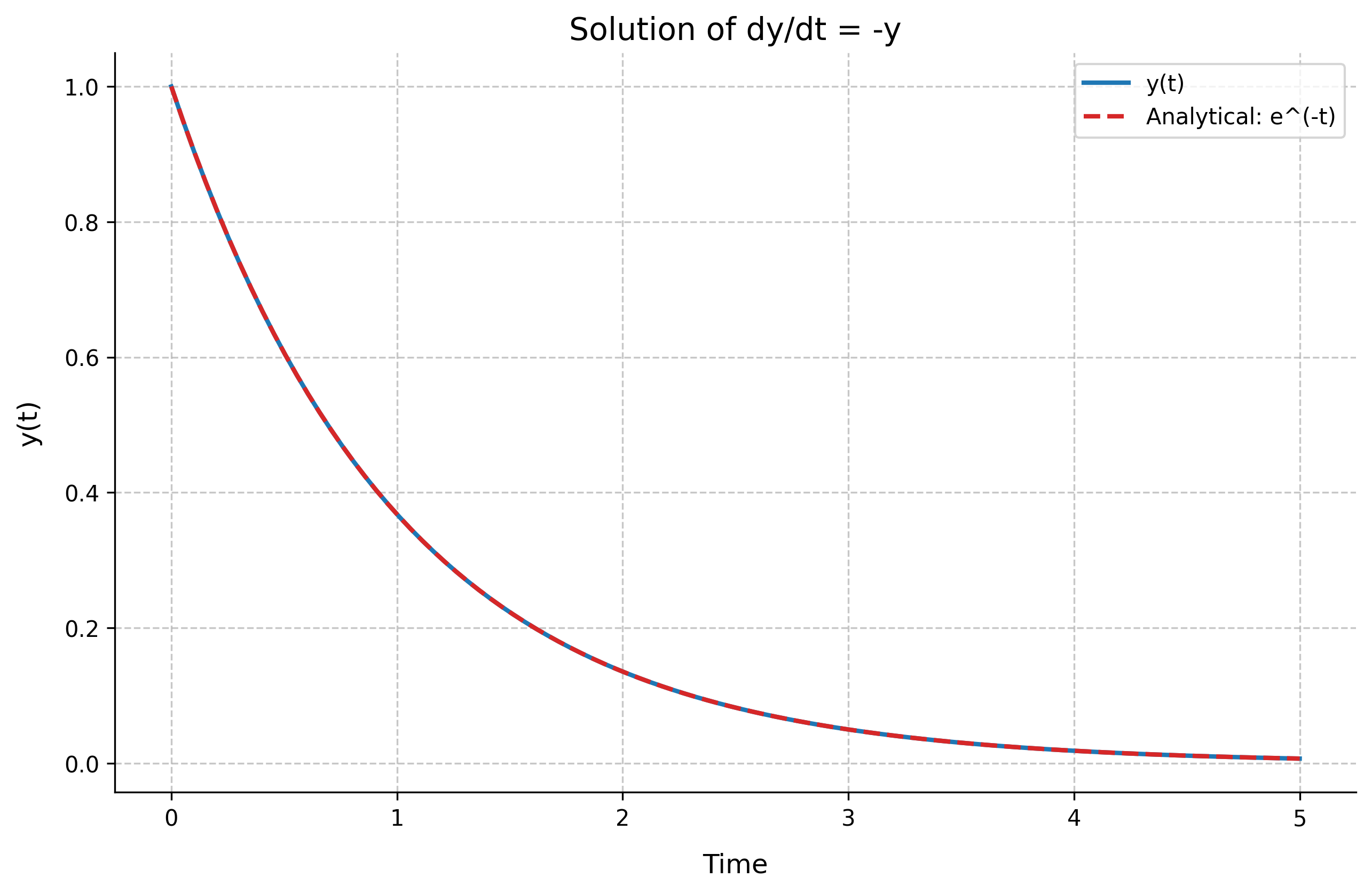
Control systems often involve differential equations. Here's how to solve them:

Consider the first-order differential equation:

\[ \frac{dy}{dt} = -y \]

With initial condition:

\[ y(0) = 1 \]

The analytical solution is:

\[ y(t) = e^{-t} \]

Solving ODEs

import numpy as np
from scipy.integrate import odeint
import matplotlib.pyplot as plt

# Define the differential equation dy/dt = -y
def model(y, t):
    return -y

# Time points and initial condition
t = np.linspace(0, 5, 100)
y0 = 1

# Solve ODE
solution = odeint(model, y0, t)

# Plot results
plt.figure(figsize=(10, 6))
plt.plot(t, solution, 'b-', label='y(t)')
plt.plot(t, np.exp(-t), 'r--', label='Analytical: e^(-t)')
plt.grid(True)
plt.xlabel('Time')
plt.ylabel('y(t)')
plt.title('Solution of dy/dt = -y')
plt.legend()
plt.show()

# Print solution values
print("Solution values at t = [0, 1, 2, 3, 4, 5]:")
t_points = [0, 1, 2, 3, 4, 5]
y_points = np.interp(t_points, t, solution.flatten())
for t_val, y_val in zip(t_points, y_points):
    print(f"t = {t_val:.1f}, y = {y_val:.4f}")

Output:

Solution values at t = [0, 1, 2, 3, 4, 5]:
t = 0.0, y = 1.0000
t = 1.0, y = 0.3680
t = 2.0, y = 0.1354
t = 3.0, y = 0.0498
t = 4.0, y = 0.0183
t = 5.0, y = 0.0067

Differential Equation Solution

Advanced Plotting Techniques

Multiple Plots and Subplots

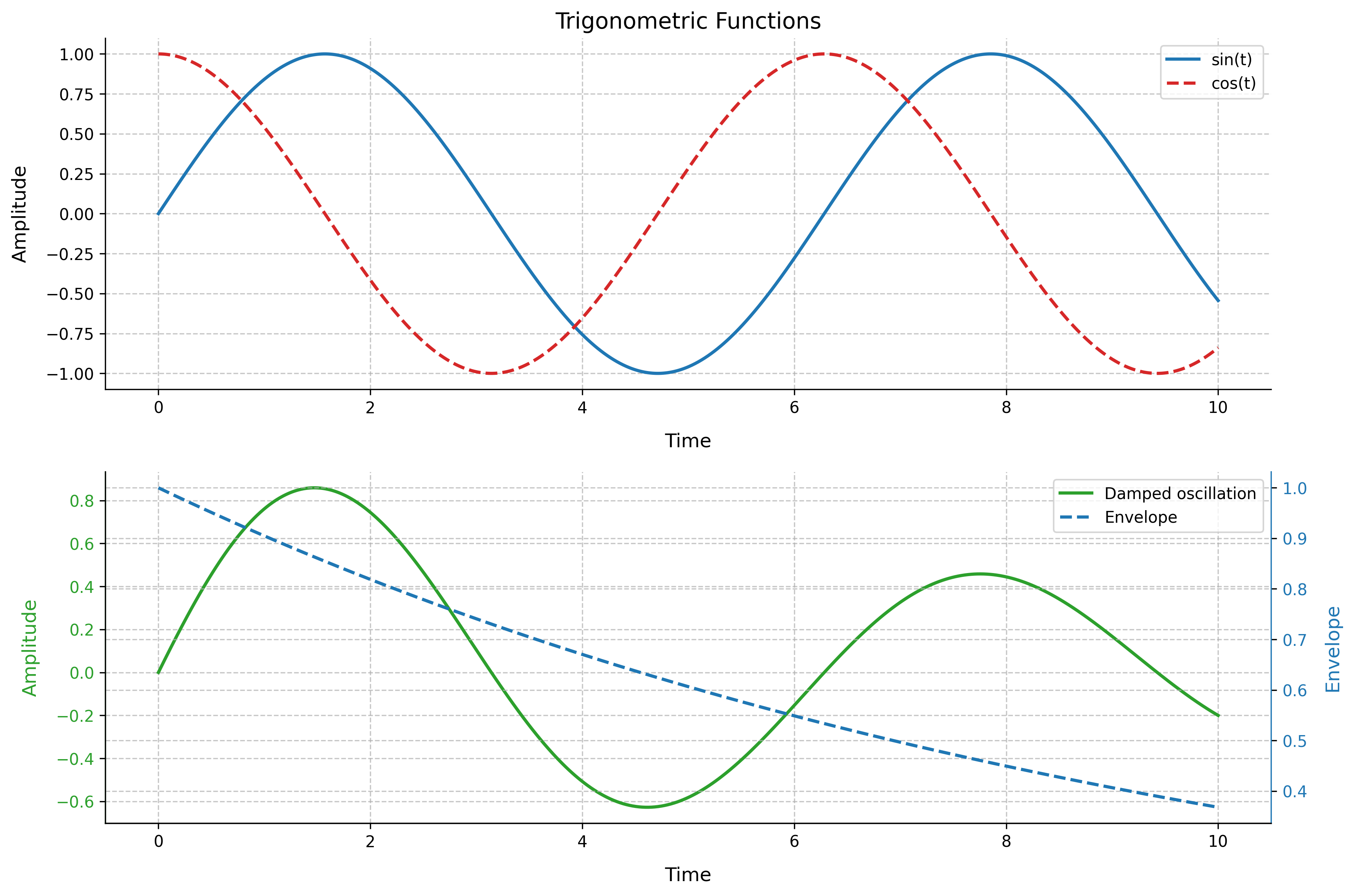
Creating Complex Plots

Control system analysis often requires multiple plots:

import numpy as np
import matplotlib.pyplot as plt

# Generate data
t = np.linspace(0, 10, 1000)
f1 = np.sin(t)
f2 = np.cos(t)
f3 = np.exp(-0.1*t)*np.sin(t)

# Create figure with subplots
fig, (ax1, ax2) = plt.subplots(2, 1, figsize=(12, 8))

# First subplot: Multiple functions
ax1.plot(t, f1, 'b-', label='sin(t)')
ax1.plot(t, f2, 'r--', label='cos(t)')
ax1.grid(True)
ax1.set_xlabel('Time')
ax1.set_ylabel('Amplitude')
ax1.set_title('Trigonometric Functions')
ax1.legend()

Multiple Plots Example

Data Visualization with Scatter Plots

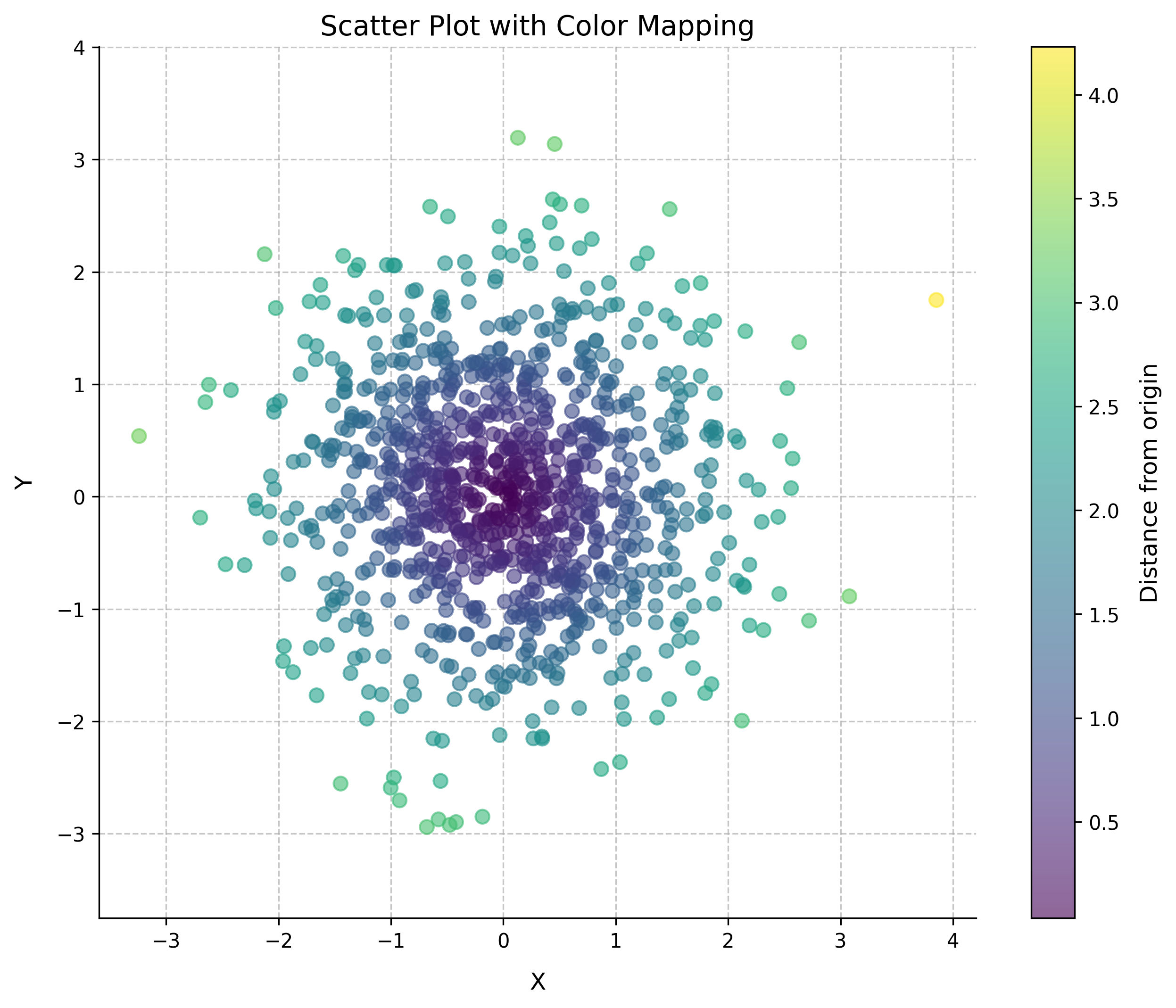
Scatter Plot with Color Mapping

Visualize relationships between variables:

import numpy as np
import matplotlib.pyplot as plt

# Generate random data
np.random.seed(42)
x = np.random.normal(0, 1, 1000)
y = np.random.normal(0, 1, 1000)
z = np.sqrt(x**2 + y**2)

# Create scatter plot
plt.figure(figsize=(10, 8))
scatter = plt.scatter(x, y, c=z, cmap='viridis', 
                     s=50, alpha=0.5)
plt.colorbar(scatter, label='Distance from origin')
plt.grid(True)
plt.xlabel('X')
plt.ylabel('Y')
plt.title('Scatter Plot with Color Mapping')
plt.axis('equal')
plt.show()

Scatter Plot Example

Control Systems with Python Control

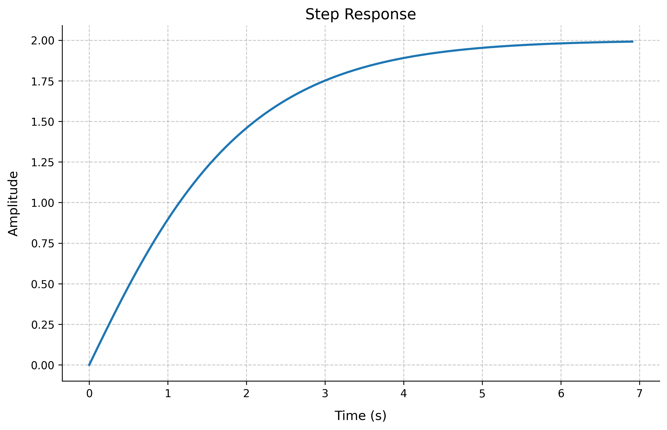
Transfer Functions and Step Response

Basic Control System Analysis

The control library provides essential tools:

Consider the transfer function:

\[ G(s) = \frac{s + 2}{s^2 + 2s + 1} \]

import control
import numpy as np
import matplotlib.pyplot as plt

# Create a transfer function G(s) = (s + 2)/(s^2 + 2s + 1)
s = control.TransferFunction.s
G = control.TransferFunction([1, 2], [1, 2, 1])

# Generate and plot step response
t, y = control.step_response(G)
plt.figure(figsize=(10, 6))
plt.plot(t, y, linewidth=2)
plt.grid(True)
plt.title('Step Response')
plt.xlabel('Time (s)')
plt.ylabel('Amplitude')
plt.show()

Step Response

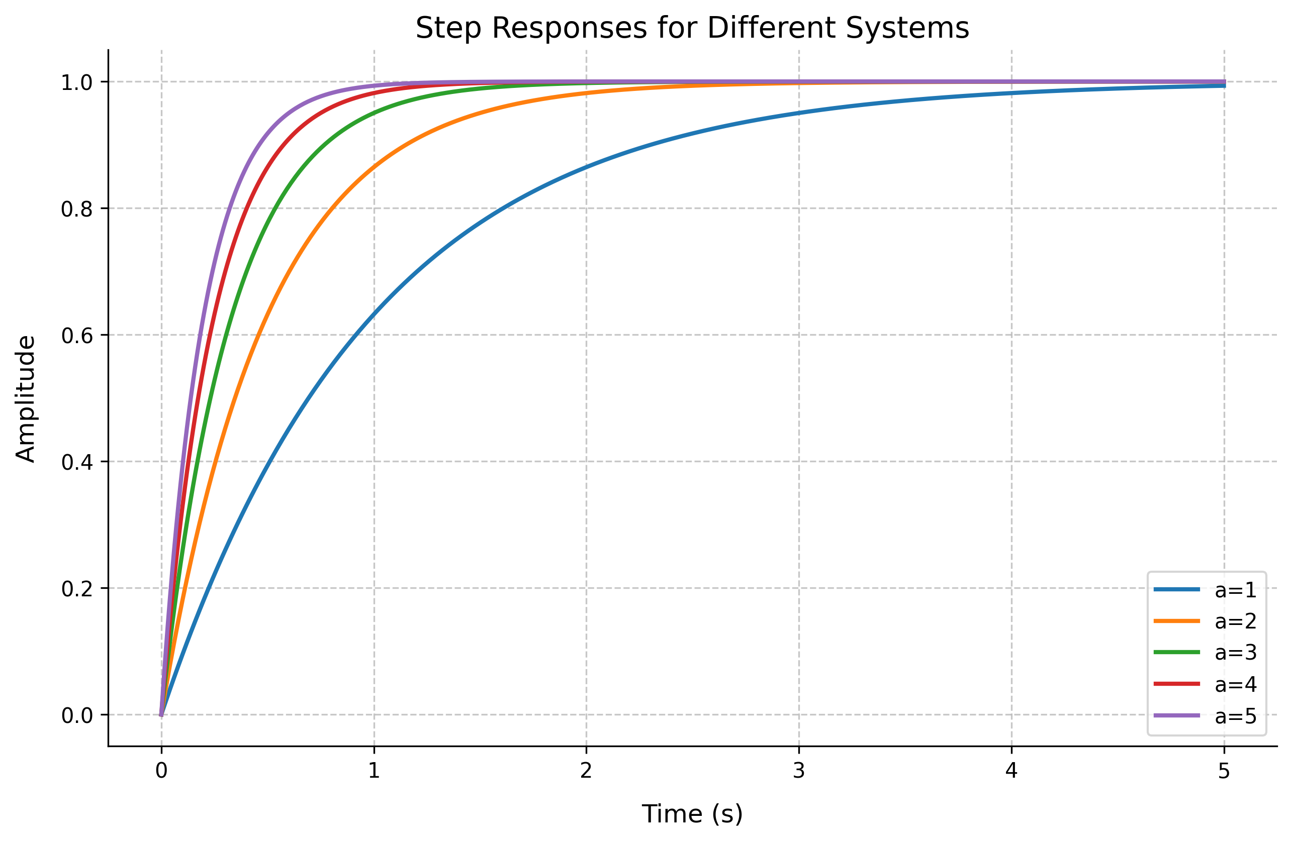
Multiple System Responses

Comparing Different Systems

Compare responses of different transfer functions:

\[ \text{For different values of } a\text{, consider: } G(s) = \frac{a}{s + a} \]

# Create multiple transfer functions
plt.figure(figsize=(10, 6))
t = np.linspace(0, 5, 500)

for a in range(1, 6):
    G = control.TransferFunction([a], [1, a])
    t, y = control.step_response(G, t)
    plt.plot(t, y, linewidth=2, label=f'a={a}')

plt.grid(True)
plt.xlabel('Time (s)')
plt.ylabel('Amplitude')
plt.title('Step Responses for Different Systems')
plt.legend(loc='lower right')
plt.show()

Multiple Step Responses

Best Practices

When working with control systems in Python:

Always use descriptive variable names
Include proper axis labels and titles
Add legends when plotting multiple curves
Use appropriate time scales for system responses
Document transfer functions and system parameters
Include grid lines for better readability
Save high-resolution figures for documentation